Coulomb’s law

When there are two point charges at rest in space, each one will feel a force proportional to the product of the two charges and inversely proportional to the squared distance between them:

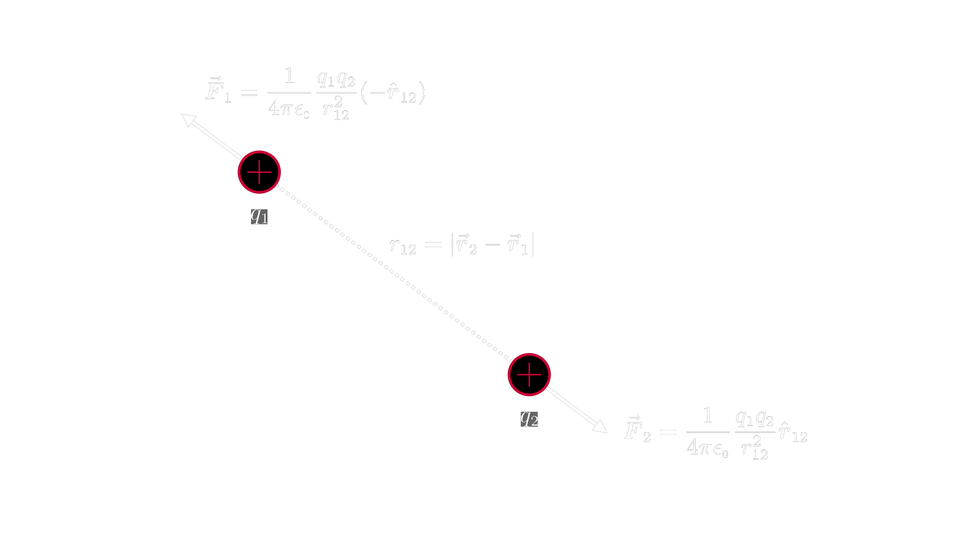
where $r_{12}$ is the distance between the charges, $\hv r_{12} = \v r_{12} / | \v r_{12}|$ is the unit vector in the direction from $q_1$ to $q_2$, and $1 / 4\pi\eo$ is a constant of proportionality, with $\eo = 8.85 \cdot 10^{-12} \; \t C^2 / \t N \t m^2$ (the permittivity of free space). The forces are equal in magnitude and opposite in direction, $\v F_1 = -\v F_2$. This is an empirical law. It describes the fundamental electrostatic interaction between point charges at rest.

Coulomb’s law obeys superposition. When there are many charges, the total force on any one charge is equal to the vector sum of its Coulomb interactions with all the other charges in the system.

The general “gist” of all problems in electrostatics is to find the force on some charge, given some existing distribution of charges. We sometimes use the term source charges to describe the given charges and test charge to describe the one we’re interested in.

In electrostatics we assume the source charges are fixed. However in general both the source and test charges can move (electrodynamics).

Vector fields; Coulomb’s law as a force field

The Coulomb force is a position-dependent force, i.e. $\v F = \v F(\v r)$. At every point in space the force vector on a particular test charge will have a unique identity that depends solely on its position relative to the other charges in the system.

When you assign a vector to each point in space you get a vector field. One way to visualize vector fields is by drawing little vector arrows at discrete points in space:

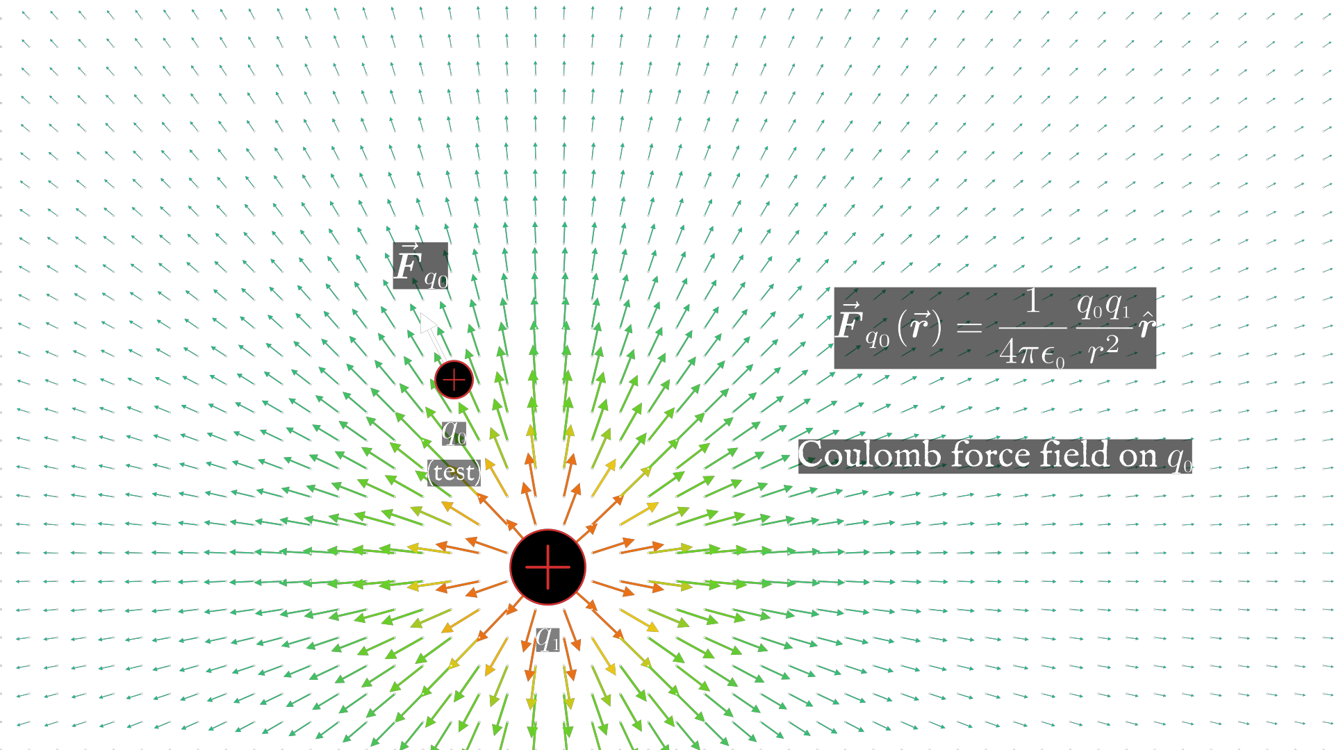
This vector field is an example of a force field. The arrows give a (crude) representation of the force that the test charge ($q_0$) would feel if it were placed at any of these points. The direction and magnitude of the force at a particular point depends on both the configuration of source charges (their positions and values) and on the value of the test charge.

Electric field

If you take the Coulomb force and divide it by the value of the test charge, you’re left with an expression that depends only on the source charges in the system. This is what we define as the electric field.

For some set of $N$ source charges $q_1, …, q_N$ and a test charge $q_0$, the electric field is:

$$\v E(\v r_0) = \frac{\v F(\v r_0)}{q_0} = \frac{1}{4\pi\eo} \sum_{j=1}^N \frac{q_j}{r_{j0}^2} \hv r_{j0}$$

The electric field is also a vector field. It’s more general than the field generated by Coulomb’s law, since it no longer depends on a specific test charge.

What the electric field gives you is the force that a unit charge would feel at a point in space, as a result of the source charge(s) in the system.

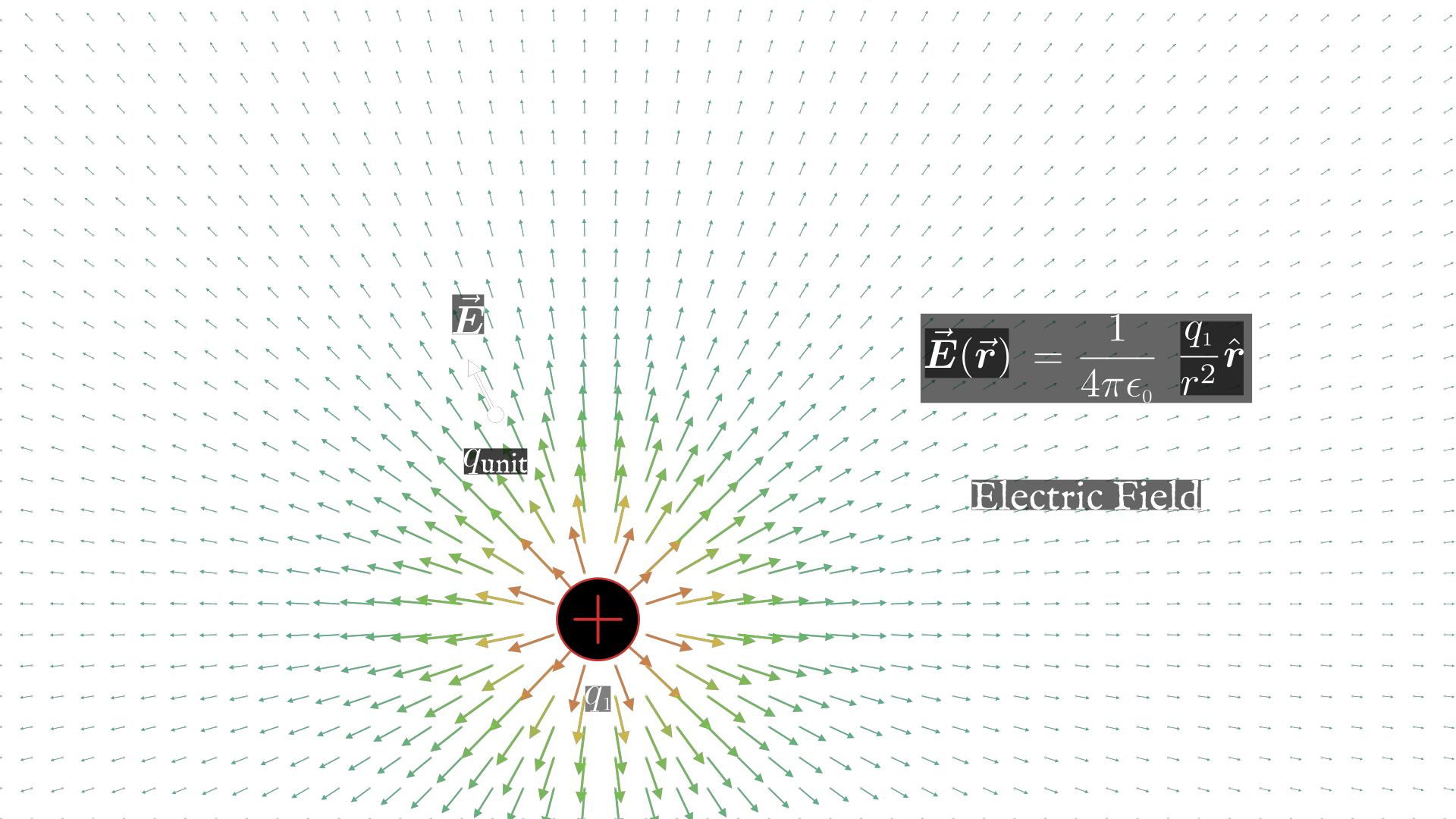
The electric field is useful because it allows us to define intrinsic properties about the field surrounding charges, e.g. that field lines always point away form positive charges and towards negative charges:

Work; line integrals

Now suppose you want to move a charge from one point to another. Some work has to be done. Here’s a (very) brief review.

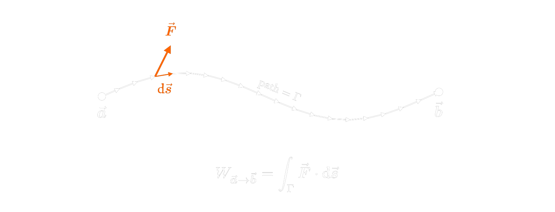
Whenever a force moves an object, we say that the force does work. If the force is uniform, the work is just equal to force times distance, $W = Fd$. If the force is not uniform (as indeed it’s not in electostatics), we can write a more general expression for work as the line integral of the force, taken over the path the object follows:

$$W = \underset{\text{path}}{\underset{\text{along}}{\int}} \v F \cdot \d \v s$$

If you’re unfamiliar with this notation, what it’s doing is dividing up the path into infinitesimal path segments, denoted $\d \v s$, then computing $\v F \cdot \d \v s$ (dot product of force with the infinitesimal path vector) for each segment, and then adding them all up. The upshot is that when you take a line integral of a force over some path, you get the work done by that force over that path.

Electric potential

Electric potential has to do with the work done in moving a charge from one point in space to another.

Suppose there’s some test charge lying about in space, initially very far away from the source charge. Let’s call this initial position the reference point, and label it $\v r_\O$. Now suppose we want to move it to some other point, closer to the source, which we’ll label $\v r$. The work done along this path is:

$$W_{\v r_{\mathcal O} \rightarrow \v r} \;\; = \;\; -\int_{\v r_{\mathcal O}}^{\v r} \v F \cdot \d \v s \label{electrostaticWork}$$

If you’re baffled by the appearance of the negative sign, the reasoning is that in order to move a charge from some point that’s far away from the source, to another point that’s less far away from the source, you have to do work against the electric field, and against the electrostatic force. Another way of saying this: as the charge moves along the path from $\v r_\O$ to $\v r$, the electrostatic force does negative work. Hence the negative sign on the integral.

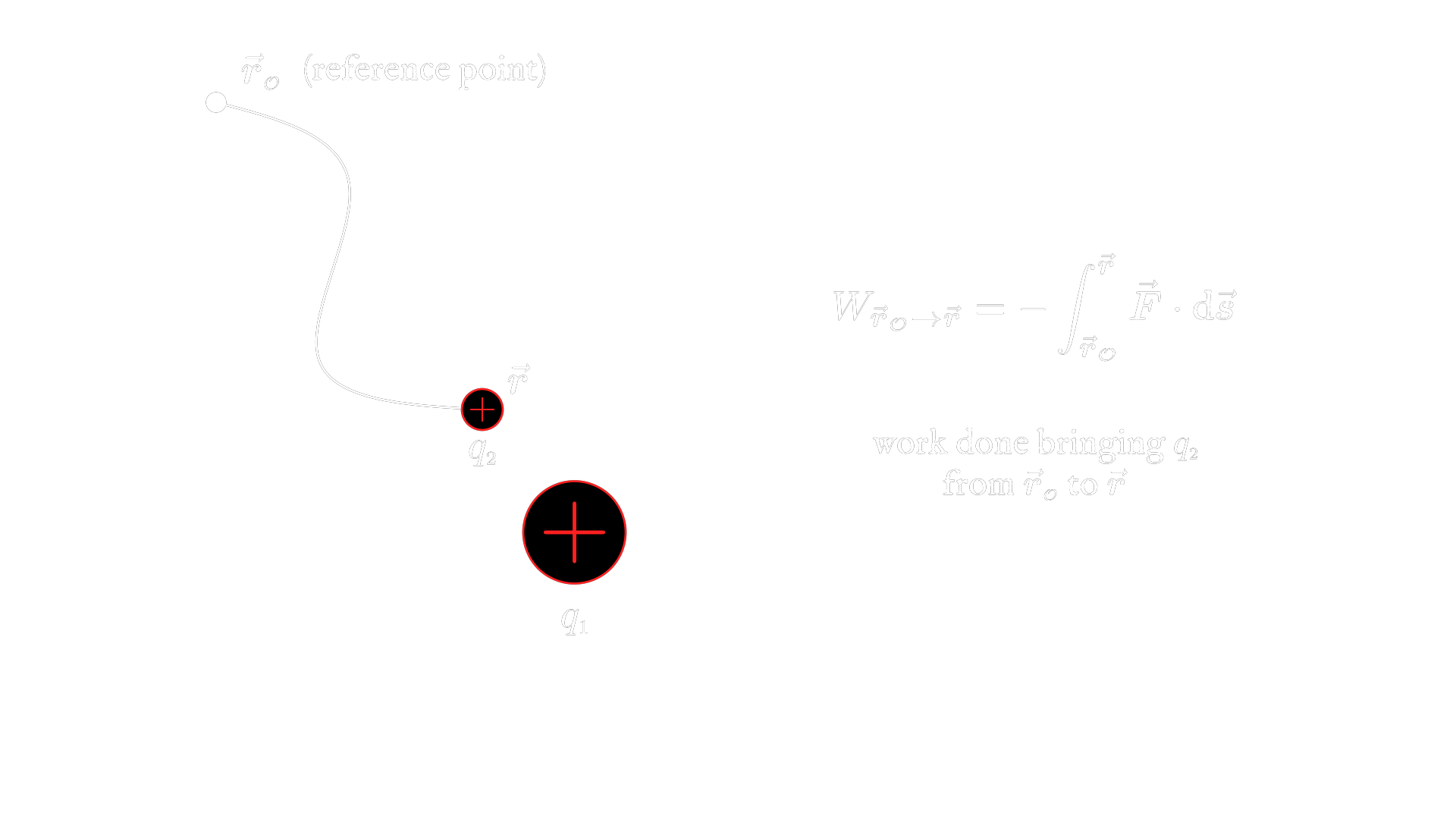
Equation $\eqref{electrostaticWork}$ gives the work done by the electrostatic force to move the test charge ($q_2$) from $\v r_{\mathcal O}$ to $\v r$. To make this expression more general, we can divide it by the value of $q_2$, to lose the dependency on the specific test charge. The resulting expression is what we define as the electric potential:

$$V(\v r) = \frac{W_{r_{\mathcal O} \rightarrow \v r}}{q_2} = -\int_{r_{\mathcal O}}^{\v r} \v E \cdot \d \v s$$

Specifically, the electric potential at a point is defined as the work done in bringing the unit charge from some reference point to the specified point.

If you evaluate the integral you’ll find that electric potential is a scalar quantity. And since it’s a position-dependent function, it can be defined for all space. When you assign a scalar to each point in space, you get a scalar field.

One common way to visualize scalar fields is using “heatmaps” or “colormaps”. Since the potential at a point is just a number, it’s easy to map to a color parameter like opacity. Another way to visualize scalar fields is by connecting up points that have the same values. The lines you end up with are called equipotentials.